4.13
(2004-5-23)
With Python
code
Pythonで解くcode を下に示す。
discount factor は、年複利とした。
連立方程式は、numpy.linalg.solve()で解いた。
# 4.13.py
# created on 2016-12-09

import numpy
import matplotlib.pyplot as plt

# input
s_percent = numpy.array([7.67, 8.27, 8.81, 9.31, 9.75, 10.16, 10.52, 10.85])
x = numpy.array([ 500,  900,  600,  500,  100,   100,   100,    50])
t = numpy.arange(len(x)) + 1
p1 =  65.95
d1 =   7.07
p2 = 101.66
d2 =   3.80

# calculate
s  = s_percent / 100 # in decimal form
st = s * t
df  = 1/(1+s)**t
df2 = 1/(1+s)**(t+1)
dx = df * x
pv = sum(dx)
txd = t * x * df2
sumtxd = sum(txd)
duration = sumtxd / pv

a = numpy.array([[p1,             p2], \
                 [p1*d1,       p2*d2]])
b = numpy.array( [pv,    pv*duration] )
x1, x2 = numpy.linalg.solve(a, b)

# output
print('4.13.py')
fmt1='{:>10}{:>10}{:>10}{:>10}{:>10}{:>10}'
fmt2='{:10}{:10.4f}{:10.3f}{:10.0f}{:10.2f}{:10.2f}'
print(fmt1.format('t', 's', 'd', 'x', 'x*d', '-PV\''))
print(60 * '-')
for i in range(len(s)):
  print(fmt2.format(t[i], s[i], df[i], x[i], dx[i], txd[i]))
print(60 * '-')
print('{:40}{:3}{:7.2f}{:10.2f}'.format('','PV=', pv, sumtxd))
print(60 * '-')
print('{:50}{:>5}{:5.2f}'.format('', 'D=', duration))
print()
print('P1 x1    + P2 x2    = PV')
print('P1 D1 x1 + P2 D2 x2 = PV D')
print('-> x1 = {:.2f}, x2 = {:.2f}'.format(x1, x2))

# plot
x  = numpy.array([-30, 40])
y1 = (pv - p1 * x ) / p2
y2 = (pv * duration - p1 * d1 * x) / p2 / d2

plt.plot(x, y1, label='P1x1+P2x2=PV')
plt.plot(x, y2, label='P1D1x1+P2D2x2=PV*D')
w  = 1.5
hw = 7
fc = 'black'
plt.annotate('(-14.04, 31.13)', xy = (x1, x2), xytext = (-15, 5), \
             arrowprops=dict(width=w, headwidth=hw, facecolor=fc, shrink=0.05))
plt.title('Fig. 4.13.py')
plt.xlabel('x1')
plt.ylabel('x2')
plt.legend()
plt.grid()
plt.show()
# end of code
output
4.13.py
t s d x x*d -PV'
------------------------------------------------------------
1 0.0767 0.929 500 464.38 431.30
2 0.0827 0.853 900 767.76 1418.23
3 0.0881 0.776 600 465.74 1284.10
4 0.0931 0.700 500 350.21 1281.54
5 0.0975 0.628 100 62.80 286.12
6 0.1016 0.560 100 55.96 304.78
7 0.1052 0.496 100 49.65 314.46
8 0.1085 0.439 50 21.93 158.28
------------------------------------------------------------
PV=2238.44 5478.81
------------------------------------------------------------
D= 2.45
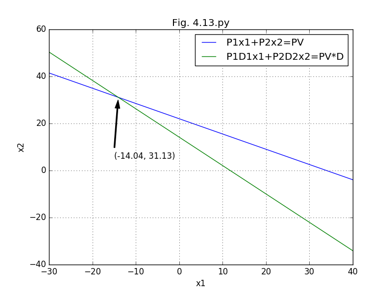
P1 x1 + P2 x2 = PV
P1 D1 x1 + P2 D2 x2 = PV D
-> x1 = -14.04, x2 = 31.13
graph
上のcodeで書いた図を下に示す。
Hand calculation
| t | st | d=1/(1+st)t | 債務 | d債務 | t債務(1+st)-(t+1) |
| 1 | 7.67 | 0.937 | 500 | 468.50 | 431.301 |
| 2 | 8.27 | 0.853 | 900 | 767.70 | 1418.235 |
| 3 | 8.81 | 0.776 | 600 | 465.60 | 1284.095 |
| 4 | 9.31 | 0.700 | 500 | 350.00 | 1281.535 |
| 5 | 9.75 | 0.628 | 100 | 62.80 | 286.116 |
| 6 | 10.16 | 0.560 | 100 | 56.00 | 304.778 |
| 7 | 10.52 | 0.496 | 100 | 49.60 | 314.464 |
| 8 | 10.85 | 0.439 | 50 | 21.95 | 158.285 |
| PV=2242.15 | 5478.809 | ||||
| デュレーションD=2.44 |
価格P1=65.95、デュレーションD1=7.07、
単位数x1
価格P2=101.66、デュレーションD2=3.80、
単位数x2
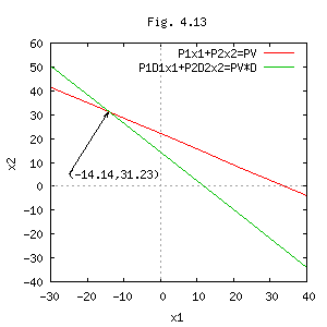
上記は、次の連立方程式を満たす。
P1x1+P2x2=PV
P1D1x1+P2D2x2
=PV*D
∴ x1=-14.14、x2=31.23
上記の連立方程式のグラフをFig. 4.13に示す。(2005-2-15)
図化コマンドを次のリンクに示す。(2011-10-26)
Julia
Juliaのコードを次のリンクに示す。
- 2023-05-03 4.13.jl
JavaScript
2024-11-02 4.13.js
Fortran
2024-11-02 4.13.f90
history
2004-05-23 create.
2005-02-15 revise.
2011-10-26 revise.
2016-12-10 add a Python code.
2021-02-17 change XHTML to html5, change shift-jis to utf-8, add viewport.
2023-05-03 add a Julia code.
2024-11-02 add a JavaScript code and a Fortran code.