4.4
解法の説明
- 債券の額面(face value) F はすべて1000($)とする。
- 表4.6の1行目の債券を b0 と呼ぶ。他も同様。
- 最後の利払いからの経過日数
number_of_days_since_last_coupon
= (2011-11-5) - (2011-08-15)
= 82(days)
- 現在の利払い期間の日数
number_of_days_in_current_coupon_perod
= (2012-2-15) - (2011-08-15)
= 184(days)
- 債券 b0 の価格
= 額面* 売値
= (face value) * (ask price)
= 1000 * 100.00(%)
= 1000($)
- 債券 b0 のクーポン額
coupon amount
= C/m = 額面 * クーポン率 / 2
= (face value) * (coupon rate) / 2
= 1000 * 6.625 / 100 / 2
= 33.13($)
ただし、mは1年あたりのクーポン支払回数(the number of coupon payments per year) - 債券 b0 の経過利息, accrued interest, AI
AI = 最後の利払いからの経過日数 / 現在の利払い期間の日数 * クーポン額
= 82 / 184 * 33.13 = 14.76($)
- 債券 b0 の総価格,
total price
= 価格 + 経過利息(AI)
= 1000 + 14.76
= 1014.76($)
債券のキャッシュフロー流列(cash flow stream), cfi は、次の通りとなる。 ただし、小数点以下は、見易さを優先するために、切り捨てで表示する。
cf0  = (-1014, 33+1000)
cf1  = (-1027, 45+1000)
cf2  = (-1025, 39, 39+1000)
cf3  = (-1028, 41, 41+1000)
cf4  = (-1030, 41, 41, 41+1000)
cf5  = (-1032, 41, 41, 41+1000)
cf6  = (-1025, 40, 40, 40, 40+1000)
cf7  = (-1039, 43, 43, 43, 43+1000)
cf8  = ( -996, 34, 34, 34, 34, 34+1000)
cf9  = (-1042, 44, 44, 44, 44, 44+1000)
cf10 = ( -989, 34, 34, 34, 34, 34, 34+1000)
cf11 = (-1036, 43, 43, 43, 43, 43, 43+1000)
cf12 = (-1008, 38, 38, 38, 38, 38, 38, 38+1000)
cf13 = (-1116, 56, 56, 56, 56, 56, 56, 56+1000)
cf14 = (-1033, 42, 42, 42, 42, 42, 42, 42, 42+1000)
cf15 = (-1101, 52, 42, 42, 42, 42, 42, 42, 42+1000)
cf16 = (-1011, 39, 39, 39, 39, 39, 39, 39, 39, 39+1000)
cf17 = (-1049, 44, 44, 44, 44, 44, 44, 44, 44, 44+1000)
上のキャッシュフローを、
総価格 = 各クーポンの現在価値 + 満期時入金の現在価値
の等式に書き換えて、次の各式を得る。ただし、d(ti)は割引係数である。
1014 = 1033d(t0)
1027 = 1045d(t0)
1025 =   39d(t0)+1039d(t1)
1028 =   41d(t0)+1041d(t1)
1030 =   41d(t0)+  41d(t1)+1041d(t2)
1032 =   41d(t0)+  41d(t1)+1041d(t2)
1025 =   40d(t0)+  40d(t1)+  40d(t2)+1040d(t3)
1039 =   43d(t0)+  43d(t1)+  43d(t2)+1043d(t3)
 996 =   34d(t0)+  34d(t1)+  34d(t2)+  34d(t3)+1034d(t4)
1024 =   44d(t0)+  44d(t1)+  44d(t2)+  44d(t3)+1044d(t4)
 989 =   34d(t0)+  34d(t1)+  34d(t2)+  34d(t3)+  34d(t4)+1034d(t5)
1036 =   43d(t0)+  43d(t1)+  43d(t2)+  43d(t3)+  43d(t4)+1043d(t5)
1008 =   38d(t0)+  38d(t1)+  38d(t2)+  38d(t3)+  38d(t4)+  38d(t5)+1038d(t6)
1116 =   56d(t0)+  56d(t1)+  56d(t2)+  56d(t3)+  56d(t4)+  56d(t5)+1056d(t6)
1033 =   42d(t0)+  42d(t1)+  42d(t2)+  42d(t3)+  42d(t4)+  42d(t5)+  42d(t6)+1042d(t7)
1101 =   52d(t0)+  52d(t1)+  52d(t2)+  52d(t3)+  52d(t4)+  52d(t5)+  52d(t6)+1052d(t7)
1011 =   39d(t0)+  39d(t1)+  39d(t2)+  39d(t3)+  39d(t4)+  39d(t5)+  39d(t6)+  39d(t7)+1039d(t8)
1049 =   44d(t0)+  44d(t1)+  44d(t2)+  44d(t3)+  44d(t4)+  44d(t5)+  44d(t6)+  44d(t7)+1044d(t8)
上の式を、次の形式で表現する。
{y} = [W]{β}
ただし、{y}は、(1014 1027 ... 1049)の転置ベクトル、{β}は、
(d(t0) d(t1) ... d(t8))の転置ベクトル、
そして、行列[W]は、
┌                                            ┐
│1033    0    0   0     0    0    0    0    0│
│1045    0    0   0     0    0    0    0    0│
│  39 1039    0   0     0    0    0    0    0│
│  41 1041    0   0     0    0    0    0    0│
│  41   41 1041   0     0    0    0    0    0│
│  41   41 1041   0     0    0    0    0    0│
│  40   40   40 1041    0    0    0    0    0│
│  43   43   43 1043    0    0    0    0    0│
│  34   34   34   34 1034    0    0    0    0│
│  44   44   44   44 1044    0    0    0    0│
│  34   34   34   34   34 1034    0    0    0│
│  43   43   43   43   43 1043    0    0    0│
│  38   38   38   38   38   38 1038    0    0│
│  56   56   56   56   56   56 1056    0    0│
│  42   42   42   42   42   42   42 1042    0│
│  52   52   52   52   52   52   52 1052    0│
│  39   39   39   39   39   39   39   39 1039│
│  44   44   44   44   44   44   44   44 1044│
└                                            ┘
である。
上の {y}=[W]{β}の{β}をPythonのnumpyのlinalg.lstsq(最小二乗法)で求め、 その結果βi=d(ti)とtiを下表に示す。
| i | ti(year) | βi =d(ti) |
| 0 | 0.279 | 0.982 |
| 1 | 0.778 | 0.949 |
| 2 | 1.282 | 0.913 |
| 3 | 1.778 | 0.877 |
| 4 | 2.282 | 0.840 |
| 5 | 2.778 | 0.804 |
| 6 | 3.282 | 0.771 |
| 7 | 3.778 | 0.740 |
| 8 | 4.282 | 0.712 |
d(t)=e-r(t)tから、r(t)は次式となる。
r(t)=-log(d(t))/t
tiと上式から求めたr(ti)を下表に示す。
| i | ti(year) | r(ti) |
| 0 | 0.279 | 0.0638 |
| 1 | 0.778 | 0.0672 |
| 2 | 1.282 | 0.0707 |
| 3 | 1.778 | 0.0737 |
| 4 | 2.282 | 0.0763 |
| 5 | 2.778 | 0.0781 |
| 6 | 3.282 | 0.0792 |
| 7 | 3.778 | 0.0794 |
| 8 | 4.282 | 0.0790 |
上表のtiとriから、 次の多項式の係数を最小二乗法で求める。
r(t) = a0 + a1t + a2t2 + a3t3 + a4t4
r(t)の多項式の係数を求めるにあたり、 tiとr(ti)の関係を次式で表し、 r(t)の多項式の係数を最小二乗法で推定する。
{y2} = [W2]{β2}
ただし、
{y2}=
| • |
| ri(ti) |
| • |
=
| 0.0638 |
| 0.0672 |
| 0.0707 |
| 0.0737 |
| 0.0763 |
| 0.0781 |
| 0.0792 |
| 0.0794 |
| 0.0790 |
[W2]=
| • | • | • | • | • |
| 1 | ti | ti2 | ti3 | ti4 |
| • | • | • | • | • |
=
| 1.000 | 0.279 | 0.078 | 0.022 | 0.006 |
| 1.000 | 0.778 | 0.605 | 0.471 | 0.367 |
| 1.000 | 1.282 | 1.644 | 2.108 | 2.703 |
| 1.000 | 1.778 | 3.162 | 5.622 | 9.996 |
| 1.000 | 2.282 | 5.208 | 11.887 | 27.127 |
| 1.000 | 2.778 | 7.718 | 21.441 | 59.564 |
| 1.000 | 3.282 | 10.773 | 35.358 | 116.053 |
| 1.000 | 3.778 | 14.274 | 53.928 | 203.744 |
| 1.000 | 4.282 | 18.337 | 78.523 | 336.252 |
{β2}=
| a0 |
| a1 |
| a2 |
| a3 |
| a4 |
∴estimated{β2} =
| 0.0621 |
| 0.00607 |
| 0.00125 |
| -0.000638 |
| 0.0000540 |
(注 βの最小二乗推定には、 Python の numpyのlinalg.lstsq(最小二乗法)を用いた。)
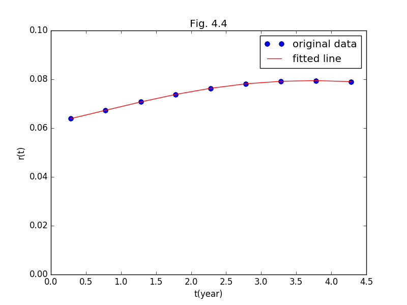
よって期間構造の推定式は、次式となる。
r(t) = 0.0621 + 0.00607t + 0.00125t2 - 0.000638t3
+ 0.0000540t4
期間構造カーブとその基データをFig.4.4に示す。
解法の解説1
1)
債券のキャッシュフローから債券の現在価値の方程式
Pi = Σci(tj) d(tj)
ただし、
Piは債権iの総価格、
ci(tj)は債券iの時点tjのキャッシュフロー、
d(tj)は時点tjに対する割引係数である。
を作成する。
この方程式を各債券に対して作成し、連立方程式にする。
P0 = c0(t0)d(t0) + … + c0(t8)d(t8) .
.
..
.
..
.
.P17 = c17(t0)d(t0) + … + c17(t8)d(t8)
上を行列表示にすると、次が得られる。
{y} = [W]{β}
ただし、
- {y}は、債券の総価格P0, ..., P17 を要素とする縦ベクトルである。{y}は、既知である。
- [W]は、債券iのd(tj)の係数ci(tj) を横に並べたものをi=0からi=17の順に縦に積み重ねた行列である。 ただし、ci(tj)は、 t = tjにおける債券iのキャッシュフローである。 [W]は、既知である。
- {β}は、d(t0), ..., d(t8) を要素とする縦ベクトルである。{β}は、未知である。
この連立方程式は、未知数が9個で、方程式が18個である。 未知数に対して方程式が多いので、方程式の解は求まらない。 そこで、最小二乗推定で未知数 d(t0), ..., d(t8)を推定する。
numpyのlinalg.lstsqを{y}と[W]に適用すると、{β}の最小二乗推定値が求まる。 すなわち、d(t0)からd(t8)の最小二乗推定値が求まる。
2)
d(t0), ..., d(t8)から連続複利のスポットレート
r(t0), ...,
r(t8)を求める。
3)
r(t)を、
r(t) = a0 + a1t + a2t2
+ a3t3 + a4t4
の形で推定するので、次の連立方程式を作成する。
r(t0) = a0 + a1t0 + a2t02 + a3t03 + a4t04
r(t1) = a0 + a1t1 + a2t12 + a3t13 + a4t14
r(t2) = a0 + a1t2 + a2t22 + a3t23 + a4t24
r(t3) = a0 + a1t3 + a2t32 + a3t33 + a4t34
r(t4) = a0 + a1t4 + a2t42 + a3t43 + a4t44
r(t5) = a0 + a1t5 + a2t52 + a3t53 + a4t54
r(t6) = a0 + a1t6 + a2t62 + a3t63 + a4t64
r(t7) = a0 + a1t7 + a2t72 + a3t73 + a4t74
r(t8) = a0 + a1t8 + a2t82 + a3t83 + a4t84
この連立方程式は、未知数aiが5個、方程式が9個である。 未知数の数より方程式の数が多いため、未知数は求まらない。 そこで、未知数aiを最小二乗推定する。 上の連立方程式を次の行列表示にする。
{r(ti)}
=[1 ti ti2 ti3 ti4 in i-th row]
{ai}
この連立方程式の
{r}は既知、行列[]は既知、{ai}は未知である。
{r}と行列[]とから最小二乗推定により{ai}を求める。
解法の解説2
-
総価格{Pi}とキャッシュフロー[ci(tj)]
とから割引係数{d(ti)}の最小二乗推定値を得る。
ただし、 {Pi}=[ci(tj)]{d(tj)}、 iは行を、jは列を表す。(i=0,...,17; j=0,...,8)
{}は列ベクトルを、[ ]は行列を表す。 - {d(ti)}から、連続複利のスポットレート{r(ti)}を求める。 (i=0,...,8)
-
r(t)を次の形で推定するために、
r(t) = a0 + a1t1 + a2t2 + a3t3 + a4t4
{r(ti)} = [Wij]{aj}となる[W]を次の通り作成する。 (i=0,...,8; j=0,...,4)
[Wi] = [1 ti ti2 ti3 ti4 in i-th row]
{r(ti)}と[Wij]とから最小二乗推定値{aj}を得る。
解法の解説3
- 債券の総価格(ask price and AI)と、クーポンC/m及び額面Fの現在価値とから、 割引係数d(ti)を最小二乗推定する。
- 割引係数d(ti)から、 連続複利のスポットレートr(ti)を算定する。
- 離散データ(ti, r(ti))から連続値である r(t) = a0 + a1t1 + a2t2 + a3t3 + a4t4 の t の係数 aj を最小二乗推定する。
解法の実装 in Python 3
code
解法を実装したPython 3 のcode を次に示す。
# 4.4.numpy.py
# created on 2016-11-26
#
#

import datetime
import math
import numpy as np
import matplotlib.pyplot as plt
from pylab import axis, title, xlabel, ylabel

date = datetime.date
log  = math.log

# input
face_value = 1000
coupon_rate = np.array([6 + 5/8, 9 + 1/8, 7 + 7/8,  8 + 1/4, 8 + 1/4, \
                        8 + 3/8, 8,       8 + 3/4,  6 + 7/8, 8 + 7/8, \
                        6 + 7/8, 8 + 5/8, 7 + 3/4, 11 + 1/4, 8 + 1/2, \
                       10 + 1/2, 7 + 7/8, 8 + 7/8])

maturity = np.array([[2012, 2], [2012, 2], [2012, 8], [2012, 8], \
                     [2013, 2], [2013, 2], [2013, 8], [2013, 8], \
                     [2014, 2], [2014, 2], [2014, 8], [2014, 8], \
                     [2015, 2], [2015, 2], [2015, 8], [2015, 8], \
                     [2016, 2], [2016, 2]])

ask_price = np.array([100+ 0/32, 100+22/32, 100+24/32, 101+1/32, 101+ 7/32, \
                      101+12/32, 100+26/32, 102+ 1/32,  98+5/32, 102+ 9/32, \
                       97+13/32, 101+23/32,  99+ 5/32, 109+4/32, 101+13/32, \
                      107+27/32,  99+13/32, 103+ 0/32])

today       = date(2011, 11,  5)
last_coupon = date(2011,  8, 15)
next_coupon = date(2012,  2, 15)


# calculate
coupon = face_value * coupon_rate / 100 / 2
t = np.array([(date(2012, 2, 15) - today).days / 365, \
              (date(2012, 8, 15) - today).days / 365, \
              (date(2013, 2, 15) - today).days / 365, \
              (date(2013, 8, 15) - today).days / 365, \
              (date(2014, 2, 15) - today).days / 365, \
              (date(2014, 8, 15) - today).days / 365, \
              (date(2015, 2, 15) - today).days / 365, \
              (date(2015, 8, 15) - today).days / 365, \
              (date(2016, 2, 15) - today).days / 365])

number_of_days_since_last_coupon        = (today - last_coupon).days
number_of_days_in_current_coupon_period = (next_coupon - last_coupon).days

accrued_interest = number_of_days_since_last_coupon  \
                 / number_of_days_in_current_coupon_period \
                 * coupon

total_price = face_value * ask_price / 100 + accrued_interest

cf0 =np.array([coupon[ 0]+face_value,0,0,0,0,0,0,0,0])
cf1 =np.array([coupon[ 1]+face_value,0,0,0,0,0,0,0,0])
cf2 =np.array([coupon[ 2],coupon[ 2]+face_value,0,0,0,0,0,0,0])
cf3 =np.array([coupon[ 3],coupon[ 3]+face_value,0,0,0,0,0,0,0])
cf4 =np.array([coupon[ 4],coupon[ 4],coupon[ 4]+face_value,0,0,0,0,0,0])
cf5 =np.array([coupon[ 5],coupon[ 5],coupon[ 5]+face_value,0,0,0,0,0,0])
cf6 =np.array([coupon[ 6],coupon[ 6],coupon[ 6],coupon[ 6]+face_value, \
               0,0,0,0,0])
cf7 =np.array([coupon[ 7],coupon[ 7],coupon[ 7],coupon[ 7]+face_value, \
               0,0,0,0,0])
cf8 =np.array([coupon[ 8],coupon[ 8],coupon[ 8],coupon[ 8],coupon[ 8]+ \
               face_value,0,0,0,0])
cf9 =np.array([coupon[ 9],coupon[ 9],coupon[ 9],coupon[ 9],coupon[ 9]+ \
               face_value,0,0,0,0])
cf10=np.array([coupon[10],coupon[10],coupon[10],coupon[10],coupon[10], \
               coupon[10]+face_value,0,0,0])
cf11=np.array([coupon[11],coupon[11],coupon[11],coupon[11],coupon[11], \
               coupon[11]+face_value,0,0,0])
cf12=np.array([coupon[12],coupon[12],coupon[12],coupon[12],coupon[12], \
               coupon[12],coupon[12]+face_value,0,0])
cf13=np.array([coupon[13],coupon[13],coupon[13],coupon[13],coupon[13], \
               coupon[13],coupon[13]+face_value,0,0])
cf14=np.array([coupon[14],coupon[14],coupon[14],coupon[14],coupon[14], \
               coupon[14],coupon[14],coupon[14]+face_value,0])
cf15=np.array([coupon[15],coupon[15],coupon[15],coupon[15],coupon[15], \
               coupon[15],coupon[15],coupon[15]+face_value,0])
cf16=np.array([coupon[16],coupon[16],coupon[16],coupon[16],coupon[16], \
               coupon[16],coupon[16],coupon[16],coupon[16]+face_value])
cf17=np.array([coupon[17],coupon[17],coupon[17],coupon[17],coupon[17], \
               coupon[17],coupon[17],coupon[17],coupon[17]+face_value])

w1 = np.vstack((cf0, cf1, cf2, cf3, cf4, cf5, cf6, cf7, cf8, cf9, \
               cf10,cf11,cf12,cf13,cf14,cf15,cf16,cf17))
y1 = total_price
p1 = np.linalg.lstsq(w1, y1)
beta1 = p1[0]

r = list(map(lambda x, y: - log(x) / y, beta1, t))

w2 = np.vstack([np.ones(len(t)), t, t ** 2, t ** 3, t ** 4]).T
y2 = r
p2 = np.linalg.lstsq(w2, y2)
beta2 = p2[0]


# output
print('4.4.numpy.py')
print('{:15}{}'.format('face value',  face_value))
print('{:15}{}'.format('last_coupon', last_coupon))
print('{:15}{}'.format('today',       today      ))
print('{:15}{}'.format('next coupon', next_coupon))

print('number_of_days_since_last_coupon= ', \
       number_of_days_since_last_coupon)
print('number_of_days_in_current_coupon_period= ', \
       number_of_days_in_current_coupon_period)
print()

fmt1='{:>15}{:>15}{:>15}{:>15}{:>15}'
fmt2='{:15}{:15.2f}{:15.2f}{:15.2f}{:15.2f}'
print(fmt1.format('i', 'ask price','coupon amount','a. interest','total price'))
print(75 * '-')
for i in range(len(ask_price)):
  print(fmt2.format(i, ask_price[i], coupon[i], accrued_interest[i], \
                    total_price[i]))
print(75 * '-')
print()

print('{:>7}'.format('i'), end='')
for i in range(len(t)):
  print('{:7}'.format(i), end='')
print()
print(70 * '-')
print('{:>7}'.format('t[i]'), end='')
for i in range(len(t)):
  print('{:7.3f}'.format(t[i]), end='')
print()
print(70 * '-')
print()

print('y1, total price')
print('{:>10}{:>10}'.format('i', 'y1[i]'))
print(20 * '-')
for i in range(len(y1)):
  print('{:10}{:10d}'.format(i, int(y1[i])))
print(20 * '-')
print()

print('w1, matrix of cf(in integer) in row')
print('{:>7}'.format('i') , end='')
for i in range(len(t)):
  print('{:>6}{:1}'.format('t', i), end='')
print()
print(70 * '-')
for i in range(len(w1)):
  print('{:7}'.format(i), end='')
  for j in range(len(w1[0])):
    print('{:7}'.format(int(w1[i][j])), end='')
  print()
print(70 * '-')
print()

print('estimated beta1, d(t[i])')
print('{:>10}{:>10}'.format('i', 'beta1[i]'))
print(20*'-')
for i in range(len(beta1)):
  print('{:10}{:10.3f}'.format(i, beta1[i]))
print(20 * '-')
print()

print('estimated r(t[i])')
print('{:>10}{:>10}'.format('i','r(t[i])'))
print(20 * '-')
for i in range(len(r)):
  print('{:10}{:10.4f}'.format(i, r[i]))
print(20 * '-')
print()

print('w2, coefficent matrix')
fmt3='{:>10}{:>10}{:>10}{:>10}{:>10}{:>10}'
print(fmt3.format('i', 1, 't', 't^2', 't^3', 't^4'))
print(60 * '-')
for i in range(len(w2)):
  print('{:10}'.format(i), end='')
  for j in range(len(w2[0])):
    print('{:10.3f}'.format(w2[i][j]), end='')
  print()
print(60 * '-')
print()

print('beta2, estimated a[i] for r(t)')
print('{:>10}{:5}{:}'.format('i', '', 'a[i]'))
print(40 * '-')
for i in range(len(beta2)):
  print('{:10}{:5}{:}'.format(i, ' ', beta2[i]))
print(40 * '-')
print()

a = beta2
print()

print('estimated r(t)=', \
       a[0], '+', a[1], 't +', a[2], 't^2 +', a[3], 't^3 +', a[4], 't^4')


# plot
def f(t):
  return sum([a[i] * t ** i for i in range(len(a))])
x = t
y = r
axis(ymin = 0)
axis(ymax = 0.1)
title('Fig. 4.4')
xlabel('t(year)')
ylabel('r(t)')
plt.plot(x, y,    'o', label = 'original data', markersize = 7)
plt.plot(x, f(x), 'r', label = 'fitted line')
plt.legend()
plt.show()
output
codeの出力を次に示す。
4.4.numpy.py
face value     1000
last_coupon    2011-08-15
today          2011-11-05
next coupon    2012-02-15
number_of_days_since_last_coupon=  82
number_of_days_in_current_coupon_period=  184

              i      ask price  coupon amount    a. interest    total price
---------------------------------------------------------------------------
              0         100.00          33.12          14.76        1014.76
              1         100.69          45.62          20.33        1027.21
              2         100.75          39.38          17.55        1025.05
              3         101.03          41.25          18.38        1028.70
              4         101.22          41.25          18.38        1030.57
              5         101.38          41.88          18.66        1032.41
              6         100.81          40.00          17.83        1025.95
              7         102.03          43.75          19.50        1039.81
              8          98.16          34.38          15.32         996.88
              9         102.28          44.38          19.78        1042.59
             10          97.41          34.38          15.32         989.38
             11         101.72          43.12          19.22        1036.41
             12          99.16          38.75          17.27        1008.83
             13         109.12          56.25          25.07        1116.32
             14         101.41          42.50          18.94        1033.00
             15         107.84          52.50          23.40        1101.83
             16          99.41          39.38          17.55        1011.61
             17         103.00          44.38          19.78        1049.78
---------------------------------------------------------------------------

      i      0      1      2      3      4      5      6      7      8
----------------------------------------------------------------------
   t[i]  0.279  0.778  1.282  1.778  2.282  2.778  3.282  3.778  4.282
----------------------------------------------------------------------

y1, total price
         i     y1[i]
--------------------
         0      1014
         1      1027
         2      1025
         3      1028
         4      1030
         5      1032
         6      1025
         7      1039
         8       996
         9      1042
        10       989
        11      1036
        12      1008
        13      1116
        14      1033
        15      1101
        16      1011
        17      1049
--------------------

w1, matrix of cf(in integer) in row
      i     t0     t1     t2     t3     t4     t5     t6     t7     t8
----------------------------------------------------------------------
      0   1033      0      0      0      0      0      0      0      0
      1   1045      0      0      0      0      0      0      0      0
      2     39   1039      0      0      0      0      0      0      0
      3     41   1041      0      0      0      0      0      0      0
      4     41     41   1041      0      0      0      0      0      0
      5     41     41   1041      0      0      0      0      0      0
      6     40     40     40   1040      0      0      0      0      0
      7     43     43     43   1043      0      0      0      0      0
      8     34     34     34     34   1034      0      0      0      0
      9     44     44     44     44   1044      0      0      0      0
     10     34     34     34     34     34   1034      0      0      0
     11     43     43     43     43     43   1043      0      0      0
     12     38     38     38     38     38     38   1038      0      0
     13     56     56     56     56     56     56   1056      0      0
     14     42     42     42     42     42     42     42   1042      0
     15     52     52     52     52     52     52     52   1052      0
     16     39     39     39     39     39     39     39     39   1039
     17     44     44     44     44     44     44     44     44   1044
----------------------------------------------------------------------

estimated beta1, d(t[i])
         i  beta1[i]
--------------------
         0     0.982
         1     0.949
         2     0.913
         3     0.877
         4     0.840
         5     0.805
         6     0.771
         7     0.741
         8     0.713
--------------------

estimated r(t[i])
         i   r(t[i])
--------------------
         0    0.0639
         1    0.0673
         2    0.0708
         3    0.0738
         4    0.0763
         5    0.0781
         6    0.0792
         7    0.0794
         8    0.0791
--------------------

w2, coefficent matrix
         i         1         t       t^2       t^3       t^4
------------------------------------------------------------
         0     1.000     0.279     0.078     0.022     0.006
         1     1.000     0.778     0.605     0.471     0.367
         2     1.000     1.282     1.644     2.108     2.703
         3     1.000     1.778     3.162     5.622     9.996
         4     1.000     2.282     5.208    11.887    27.127
         5     1.000     2.778     7.718    21.441    59.564
         6     1.000     3.282    10.773    35.358   116.053
         7     1.000     3.778    14.274    53.928   203.744
         8     1.000     4.282    18.337    78.523   336.252
------------------------------------------------------------

beta2, estimated a[i] for r(t)
         i     a[i]
----------------------------------------
         0     0.062086370760156565
         1     0.006071621745898055
         2     0.0012515798717840998
         3     -0.0006384168097172578
         4     5.398054834520206e-05
----------------------------------------


estimated r(t)= 0.0620863707602 + 0.0060716217459 t + 0.00125157987178 t^2 + -0.000638416809717 t^3 + 5.39805483452e-05 t^4
既に上に示した図は、Python の codeによりプロットした図である。
JavaScript code
2024-11-02 4.4.js for node.js
Gauche code
2024-11-02 4.4.scm
Julia code
2024-11-02 4.4.jl (2024-12-07 revise, 2025-02-01 open.)
Fortran code
2024-11-02 4.4.f90 (2024-12-07 revise, 2025-02-01 open.)
history
2004-09-24 create.
2011-11-02 revised.
2016-04-04 estimation of β in Gauche added.
2016-04-09 estimations of β in gnupot and Python added.
2016-10-15 Gauche code linked.
2016-11-05 estimation of β in Maxima added.
2016-11-20 estimation of β by numpy.linalg.lstsq added.
2016-11-26 all revised for correcting d(t) function.
2021-02-17 change XHTML to html5, change shift-jis to utf-8, add viewport.
2024-11-02 add a JavaScript code, a Gauche code, a Julia code and a Fortran code.
2025-02-01 open revised 4.4.jl, revised 4.4.f90.